5 GHz Radar
So You Want to Build a Radar
Having made a couple of radios at this point, I wanted to try my hand at building a radar instead.
For the uninitiated, there a several different types of radar with varying use cases. The type that most people have heard of, and probably the thing that comes to mind when you think of a radar, is pulsed radar.
As the name suggests, a pulsed radar simply sends out a pulse and measures the time between when it was transmitted and when it “sees” its reflection come back. This is easy to understand, but there are some problems with this approach. Namely, all half duplex pulsed radars have some “blind range” where any close reflections will not be detected because the frontend is in the process of switching from TX to RX mode. This makes them generally unsuitable for measuring objects that are relatively close (in terms of the speed of light) to the transmitter.
Fortunately for us, there is another option. A more interesting architecture is the Continuous Wave (CW) radar.
CW Radars
When people talk about police radars, this is what they are referring to. Unmodulated CW radars transmit a constant tone at a fixed frequency. This tone source is split into two paths, one of which goes out over the air, while the other gets fed in as the LO source for a mixer that is fed by a receiving antenna (if you’re unfamiliar with these terms, see my page on building a radio receiver for more information).
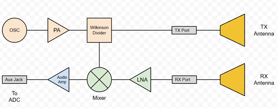
A consequence of this architecture is that CW radars are “blind” to objects that are stationary in their reference frame. All stationary reflections come back at the same frequency as the transmitted wave, and therefore get mixed down to DC. For objects in motion, the reflected wave will be doppler shifted according to the following formula where lambda is the wavelength of the TX signal:
This means that if we know what our TX wavelength is, we can very accurately determine the relative velocity of an object in our radar beam. The keyword here is relative. With just a single mixer, we can’t determine if the object is moving towards us (reflection is > TX frequency) or away from us (reflection is < TX frequency). Additionally, the measured speed will be reduced by a cosine factor that accounts for the angle between our radar beam and the target’s direction of travel:
This is great liability protection for law enforcement, as it means it’s only possible to measure you going slower than your actual speed (unless you are driving towards them directly head-on).
FMCW Radars
You might notice a problem with CW radars. Because we’re transmitting all the time, and the mixer only provides us with relative velocity information, we have no way to determine how far away our target is! If you’re a cop, this is fine, but if you’re a collision avoidance sensor, this information is critical.
Luckily there is a simple solution that, in theory, requires no changes to our existing hardware setup.
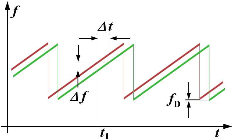
If we gradually increase (or decrease) the frequency of our transmitted tone over time, something interesting happens. When we assume a perfectly continuous and monotonic frequency ramp, any reflections showing up at the RX antenna will be at a different frequency from our current TX frequency. This means that they will not get mixed down to DC and instead show up at the output of the mixer!
It is now obvious that we can use this to map an IF frequency to a distance from the transmitter, where df/dt is the rate of change of the transmitted tone and c is the speed of light:
Practially, there are some constraints. We can’t ramp our signal forever since we’ll eventually run out of bandwidth. This puts a limit on both how far we can measure and, somewhat counterintuitively, our range resolution.
Typically the constraint for maximum range is the IF bandwidth. Once the difference in frequency between the transmitted and reflected signals falls outside the passband of our antialiasing filter, we begin to lose the ability to detect things. If our IF bandwidth is known, we can determine r_max as:
So what about range resolution? You might think that range resolution is only a function of how fast our ADC is. After all, the more points we sample at IF, the more FFT resolution we get, right? However, the range resolution of our radar is in fact entirely determined by the RF bandwidth of the TX signal:
If you want to see how this is derived, see this excellent stackoverflow response. (Not mine, just including as a good reference).
Building It
Link Budget
The first step of any RF project should be creating a link budget. This accounts for all the major sources of gain, loss, and noise, and tells you what specs your system needs to accomplish whatever you’re trying to do. Radar link budgets are extremely interesting (read: painful) because losses scale with the 4th power of distance. I.e, for an object that’s twice as far away, its radar return is 16 times weaker.
The reason for this is the fact that you have to apply the inverse square law twice. As signals spread out through space, they are effectively spread over the surface of a sphere with a radius equal to the distance from the transmitter:
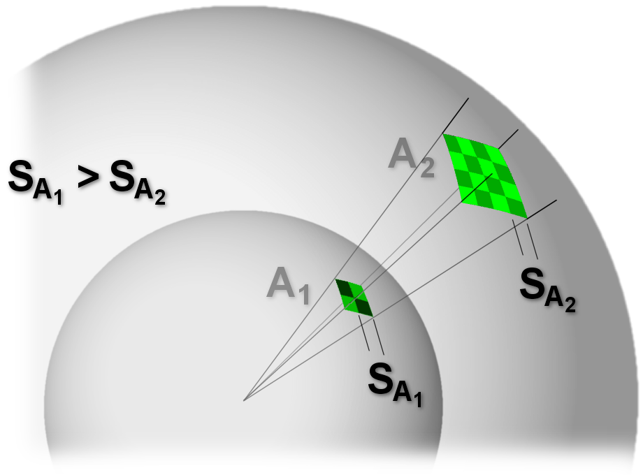
This introduces what we call “spreading loss”, as the signal strength at a given aperture at distance r is attenuated by:
Slight aside: people often refer to free space path loss when constructing link budgets. This formula often gives the wrong impression that loss over distance is higher for shorter wavelengths because it includes a wavelength term in the denominator, ex:
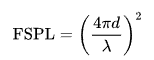
However, this is deceptive! Spreading loss is constant regardless of wavelength! This formula is attempting to account for the fact that the effective aperture size of a resonant omnidirectional antenna increases with wavelength:
You can see in the equation above that if we hold G constant at 1, Ae will decrease with wavelength. This is because as your resonant antenna gets smaller and smaller, its aperture is collecting fewer and fewer photons. This has nothing to do with what’s happening to the wave as it travels through free space!
Rant over, now back to radar.
Imagining our transmitter as a point source, its transmitted signal will spread out over the surface of a sphere. Eventually this sphere grows large enough to intersect our target. Now part of this energy gets bounced back according to the target’s radar cross section. This is the physical size the target would be if it was 100% reflective to RF energy. This means that in real life, the RCS of actual objects is always smaller than their physical size. People often say that the F35 has the RCS of a sparrow, for instance.
It follows that our reflected energy will also spread over a sphere of radius r. Combining this with the above formulas where sigma is our target RCS and Ae is the effective aperture of our RX antenna, we get:
There you have it, r^4. Physicists talk about the tyranny of the rocket equation, but I think the tyranny of the radar equation is a close second.
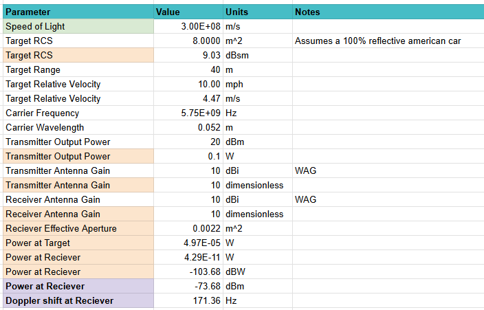
My goal for this project was to be able to measure the speed of a car at a reasonable distance, like from my balcony. Incorporating the formulas above, that produced the following link budget:
Choosing an Operating Frequency
There are a couple constraints when choosing the frequency range for a hobby radar. Here are the biggest ones that I considered
- Legality
- We must be allowed to transmit in this band with a General class ham radio license or lower
- Price
- Components cannot be prohibitively expensive.
- I (loosely) held myself to a total dev budget of $500 for this project
- Cost plus contracting also applies to personal projects
- Range + Doppler resolution
- Doppler resolution for a fixed IF bandwidth increases as frequency increases
- Range resolution increases with RF bandwidth. This means we want to operate at higher frequencies since the fractional bandwidth of a fixed size passband decreases with frequency. This makes things like filters and amplifiers easier to match.
- Testability
- VNAs and Spectrum analyzers have standard frequency range cutoffs, with higher frequency equipment becoming rarer and more expensive. For the microwave range these are usually:
- 3 GHz
- 6 GHz
- 13.6 GHz
- 26.5 GHz
- 40 GHz
- Standard SMA connectors only support up to 18 GHz, after which we must use more expensive interconnects such as 2.92mm or SMP
- VNAs and Spectrum analyzers have standard frequency range cutoffs, with higher frequency equipment becoming rarer and more expensive. For the microwave range these are usually:
- PCB Stackup Constraints
- Low cost substrates are often quite lossy
- Weave variation can start to cause undesirable effects around Ku and above
- Surface roughness and etch tolerance, among other factors, can also introduce additional headaches at high frequencies
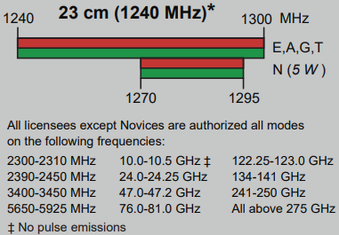
For legality, there is a helpful blurb on the ARRL band plan poster that lists out microwave bands with amateur allocations:
With component price, an interesting pattern emerges. Below I’ve plotted the price of Qorvo LNAs in the Mouser catalog in terms of price and maximum frequency:
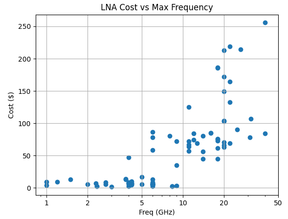
Up to 6 GHz prices are fairly reasonable because this part of the spectrum is where most consumer devices operate (WiFi, LTE, Bluetooth, etc.). Beyond this, we see a sharp increase in cost due to the increasing complexity of designing high frequency active devices in tandem with the lack of an economy of scale.
Combining all these factors, I chose to design my radar to operate in the 5.6 – 5.9 GHz band. This allows me to maximize range and doppler resolution while minimizing cost and allowing me to use the test equipment that I already have access to.
V1.0 Design
For the first version of the design, I wanted to minimize unique BOM count as much as possible. This makes ordering and assembly easier since I will be doing both by hand.
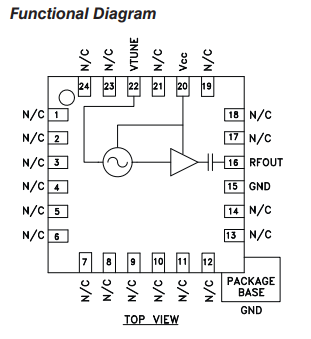
For the TX/LO source, I settled on the HMC431, which is an open loop VCO designed to operate around 5.5 – 6 GHz. It’s output power is only around +0 dBm, so we’ll need an amplifier to get enough drive strength for the LO and to give us more power over the air.
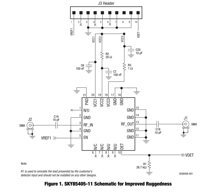
For the PA, I settled on the SKY85405-1. It’s a three stage amp originally designed for consumer WiFi routers that was perfect for my application since it’s internally matched and has > 30 dB of gain. Unfortunately, while you can order it on Mouser or DigiKey, the public datasheet includes almost no technical information, not even so much as a pinout. But after doing some digging, I found an application note with all this info that Skyworks must have forgotten to redact:
To again minimize complexity, I decided to feed both the TX output and LO input from the same source with no other amplifiers in the loop. For the Wilkinson divider, I simulated a simple design in HFSS and exported it by hand into KiCad:
This is a simple narrowband design that just uses two 70 Ohm 1/4 wave transformers and an isolation resistor to present an acceptable match at all ports. I was able to get more than enough fractional bandwidth to cover the band of interest without any fancier design tweaks to make it more wideband. Ideally the inside of the divider would also get a GND pour, but in sim this didn’t appear to make a difference.
Assembly + Bugs
V1.0 bringup went fairly smoothly, except for the fact that I accidentally placed R25 and R26 in layout such that it was possible to solder them both vertically (the correct way) and horizontally (the way I placed them). After identifying and correcting this, I was able to see a clear sine wave at the IF output when waving my hand in front of the radar.
There were a couple other goofs. I accidentally used a 1.27mm pitch header for power instead of the intended 2.54mm header. Additionally, I accidentally omitted the input matching capacitor that the datasheet recommends for both LNAs.
For simplicity, I decided to power all +5V components on the board (the PA + opamps) directly from the power header with no intermediate power stage or filtering. This ended up being a huge problem since any EMI on the power rails will couple into the IF and PA stages and create spurs in the radar spectrum. When powering from a bench PSU with good filtering this was mostly fine, but operating off of noisy USB power made the radar completely unusable.
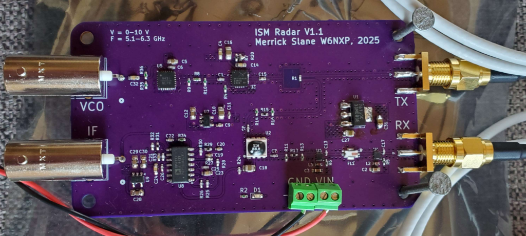
V1.1 Design
For the V1.1 design, I implemented the following fixes:
- Added a +5V high PSRR LDO connected to the power header
- Changed the power header footprint to 2.54mm
- Added an input matching cap to each LNA
- Added the option to AC couple the VCO with a series cap
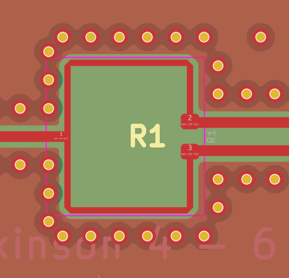
For bringup on V1.1, I decided to sacrifice one of my PCBs and a 50 ohm resistor to try and see how good my SMA match was. Connector launches on PCBs tend to have poor return loss at high frequencies unless carefully optimized in sim. I used a launch design based the results from this page by Rob Ruark (who incidentally happens to be my coworker, though I discovered his page independently!).
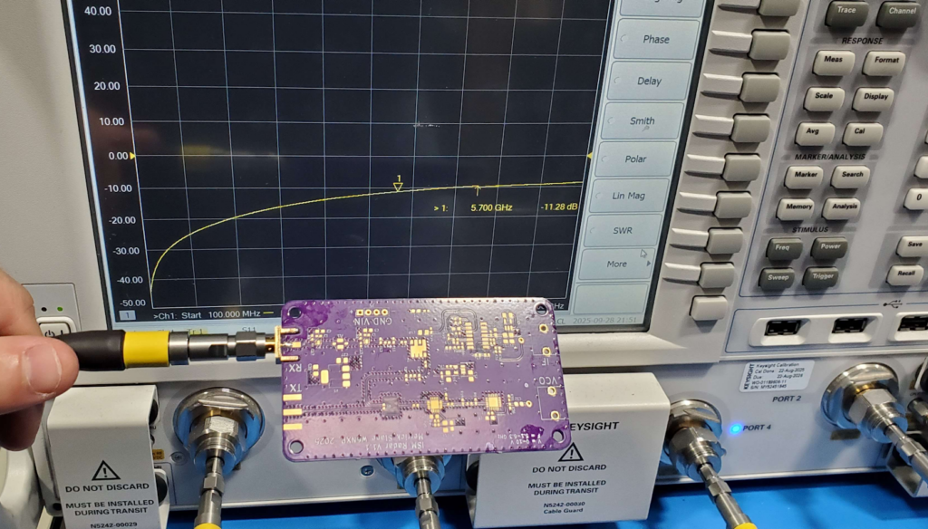
At 5.7 GHz we’re getting -11.3 dB into an 0402 resistor with a cut trace. This is not exceptional performance and at VSWR = 1.8 we could be source pulling the LNA into an undesirable noise circle. As far as personal projects go this is fine though, and it’s within the VSWR < 2 rule of thumb that hams often use. It is also worth noting that I did not do any TDR to try and see how much of this was coming from the trace/resistor vs the connector itself.
Over the Air Testing
After verifying that I could detect thrown tinfoil balls, waving hands, and my ceiling fan, I decided to give tracking cars a shot. I ordered two 5 GHz wifi yagis from Pasternack and mounted them to a scrap 2×4. I ended up orienting TX and RX at 90 degree angles to one another for polarization diversity in an effort to reduce TX -> RX desense. TBD if the increased RX sensitivity actually makes up for the polarization loss though.
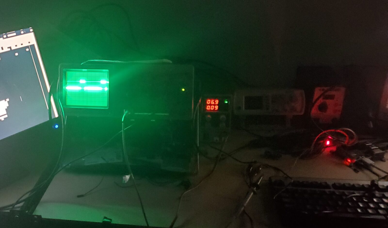
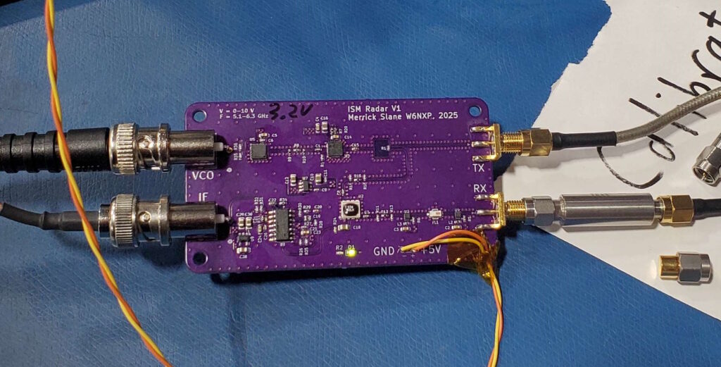
You can see my janky balcony setup below. I left the VCO input disconnected and set the resistor voltage divider to 3.2V which I measured as the approximate control voltage required for a 5.7 GHz carrier. The IF output is connected to a USB soundcard whose baseband input was then piped into SDRSharp.
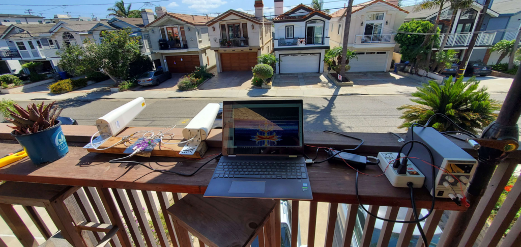
This definitely freaked out more than a couple neighbors driving by who probably thought I was trying to hack their cars or microwave their brains or something. I ended up retreating inside after I had gotten enough concerned glares for the day.
The upside is that I got some really good data! Cars are fast and have a pretty high RCS, so they make great targets for this kind of radar. You can see the waterfall plot from a particularly good pass below.
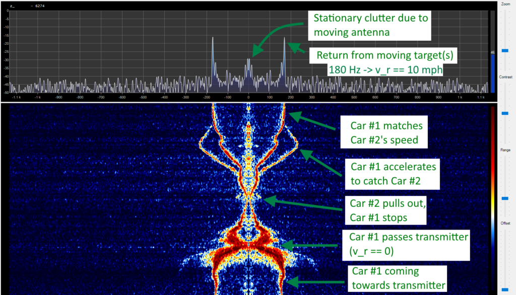
Lots of interesting information can be gleaned from this. This is an I/Q baseband waterfall plot of soundcard audio, so the spectrum on the left and the right are mirror images of one another and have redundant information. Since relative velocity is directly mapped to frequency in a CW radar, this plot is showing relative velocity (horizontal axis) vs time (vertical axis).
The signal seen near the center of the plot is a clutter return caused by me moving the antenna to track cars. When the antenna is moving, stationary objects appear to have a nonzero velocity in its reference frame, so reflections off of them don’t show up at DC and therefore are not filtered out. You can actually take advantage of this effect to measure your own velocity. A famous example of this is the landing radar used on the Apollo LEM.
The other strong signals seen in the image are radar returns off of moving cars! The plot annotations describe what is happening in the scene over time. We can tell from the two simultaneous returns that the radar had two cars in its field of view, and they were both traveling around 10 mph (4.8 m/s) at the end of the capture.
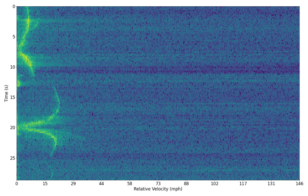
After basic testing in SDRSharp, I used a python script I had written a couple years ago to directly read in audio from the soundcard and produce velocity vs time plots in matplotlib. This spat out nice human readable plots like the one below of a Mustang Mach E and a random van driving by.
V1.2 and FMCW
Now that I had gotten a CW radar working, I wanted to move on to the next step of FMCW and get distance resolution on objects.
FMCW (Frequency Modulated Continuous Wave) radar uses a linearly increasing and/or decreasing frequency chirp to determine the distance of objects in its view. This allows us to see stationary objects and measure how far away they are.
In a system like this with a linear ramp, the frequency of a return is related to its range as follows:
Where r is the range of an object and df/dt is the frequency ramp rate of the chirp with respect to time.
However, another crucial thing to consider when building an FMCW system is the bandwidth of your chirp. Range resolution is directly related to bandwidth, and counterintuitively has absolutely nothing to do with ramp rate. See this stackoverflow post for a more detailed derivation of this. For any FMCW system, the size of each range bin is given as:
Where BW is the difference in frequency between the start and end of a single chirp.
It also logically follows that there will be a maximum detectable range based on the duration of a given chirp and the maximum detectable IF frequency.
V1.2 Design + Testing
For V1.2, I wanted to use a dedicated phase locked loop instead of an open loop VCO. The chip I ultimately settled upon was the LMX2594, as it actually has a built-in ramp generator specifically designed for FMCW radars!
Initial CW testing with this chip went smoothly, and phase noise with the PLL was much better as expected. However, when attempting my first ramps I ran into a problem. As part of its sweep logic, the LMC2594 will automatically pause to recalibrate its VCO after it has passed its programmable recalibration threshold. These pauses introduce sweep discontinuities that show up in the Radar’s output spectrum. You can increase this threshold arbitrarily by programming the sweep registers, but if you choose a value that is too large, the sweep will silently fail and produce a garbage spectrum.
I am far from the first person to have this problem, and TI has released an app note testing the largest possible calibration free sweep over temp and starting frequency.
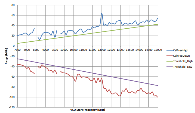
The PLL on this chip will not lock below 7500 MHz, so for operation at 5.7 GHz we need to run the VCO at 11.4 GHz and use the internal frequency divider. This will cut our usable VCO range in half relative to the value shown in this plot.
TI’s testing indicates that descending ramps have a wider achievable bandwidth than ascending ramps, so I ended up inverting the ramp direction. This has no effect on the IF spectrum. In my testing at room temperature on a single chip, I was able to reliably run a calibration free sweep at 5.7 GHz with an RF bandwidth of 150 MHz.
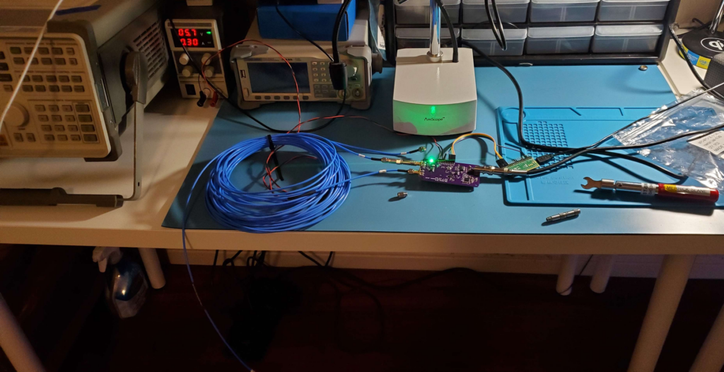
Loopback Testing
To see if my basic proof of concept worked, I tested the radar in loopback mode with a long coax cable and some high value attenuators.
In SDRSharp this produced the following spectrum:
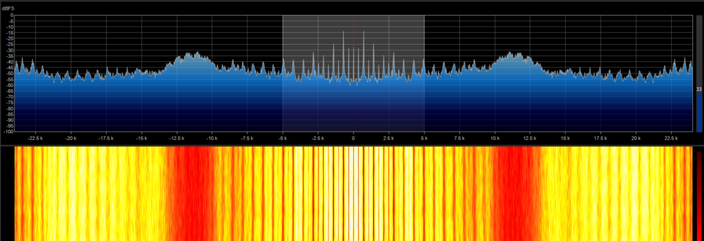
We can see that there is a peak with a ~2.5 kHz bandwidth at around 11.25 GHz. Does this make sense? I have two 8 meter cables connected together with the following manufacturer specs:
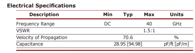
This is a loopback, so we will measure the total length of the cable divided by two (since the radar thinks it’s looking at a reflection). Doing this math for a medium with the propagation velocity of this cable, we expect to see a return centered at the following frequency:
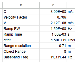
This is almost exactly what we measure in the spectrum plot! So the radar is working as expected.